Introduction
Have you ever wondered to yourself: What is the best path to draw an outline without lifting my pen? Or maybe the question was: How can I tell a robot to draw a 2D image using circles? If these questions keep you up at night like me, then look no further.
What are Epicycles?
Any image can be expressed by a series of frequencies on the 2D plane. The series of connected circles rotating is called epicycles, and a great explanation can be found here and here
Project Objectives
The objective here is: given an image, compute the contour of the image, conduct the Discrete Fourier Transform (DFT) on the path, and animate the epicycle of N circles required to compute that path. Lets go.
- Input image as coordinates (X,Y)
- Find shortest tour path of points
- DFT in series of path
- Draw circles animated
Brief Maths
I will keep the math of this post very brief. Much smarter people than me have covered this topic in depth, but the major equation to keep in mind is that to a defined order, any curve can be approximated by the form:
Where \(z(t)\) is the curve, and \(c_{j}\) is the coefficient for each order of the exponent. A true Fourier series would go to infinity, but constraints in reality force us to cut off the order to some \(m\) for approximation.
Lets Start Coding!
First, we need import some dependencies and load our image.
#Dependecies
import numpy as np
import matplotlib.pyplot as plt
import PIL
from IPython.display import HTML
from matplotlib import animation, rc
from scipy.integrate import quad

#Are you team Tau or team Pi?
tau = 2*np.pi

%matplotlib inline
#import image
im = PIL.Image.open("pi.png").convert("L")
contour_plot = plt.contour(im,levels =50,origin='image')
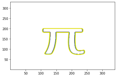
#Find path
contour_path = contour_plot.collections[0].get_paths()[0]
X, Y = contour_path.vertices[:,0], contour_path.vertices[:,1]

#Center X and Y
X = X - min(X)
Y = Y - min(Y)
X = X - max(X)/2
Y = Y - max(Y)/2

#Visualize
plt.plot(X,Y)
#For the period of time 0-2*pi
time = np.linspace(0,tau,len(X))
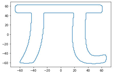
Now we have a contour of the verticies of our image! Also we have centered them around zero, which helps us with the next steps... Lets define some user functions!
def f(t, time_table, x_table, y_table):
    #Convert the X and Y coords to complex number over time
    X = np.interp(t, time_table, x_table)
    Y = 1j*np.interp(t, time_table, y_table)
    return X + Y


def coef_list(time_table, x_table, y_table, order=5):
    #Find the real and imaginary parts of the coefficients to the summation
    coef_list = []
    for n in range(-order, order+1):
        #integrate across f .
        real_coef = quad(lambda t: np.real(f(t, time_table, x_table, y_table) * np.exp(-n*1j*t)), 0, tau, limit=100, full_output=1)[0]/tau
        imag_coef = quad(lambda t: np.imag(f(t, time_table, x_table, y_table) * np.exp(-n*1j*t)), 0, tau, limit=100, full_output=1)[0]/tau
        coef_list.append([real_coef, imag_coef])
    return np.array(coef_list)

def DFT(t, coef_list, order=5):
    #Compute the discrete fourier series with a given order
    kernel = np.array([np.exp(-n*1j*t) for n in range(-order, order+1)])
    series = np.sum( (coef_list[:,0]+1j*coef_list[:,1]) * kernel[:])
    return np.real(series), np.imag(series)
Take a minute to review what these functions do...
- First, we need to convert the X and Y coordinates to Complex plane, where real numbers fall on the X axis and imaginary numbers fall on the Y axis.
- Second, We need to get the real and imaginary coefficients by the fourier transform on the original path, integrating across the time from 0 to 2\(\pi\)
-
Third is the Discrete Fourier Transform of the coefficient list.
- When the series is summed together, it is the addition of multiple circles with frequencies \(c_k\)
- What this shows is that as the order increases, the longer the fourier series is, meaning more circles to draw, the closer to the original path you become.
The last part is visualization.
Special shoutout to WirkaDKP for the great code as to how to visualize the results!
def visualize(x_DFT, y_DFT, coef, order, space, fig_lim):

    fig, ax = plt.subplots()
    lim = max(fig_lim)
    ax.set_xlim([-lim, lim])
    ax.set_ylim([-lim, lim])
    ax.set_aspect('equal')

    # Initialize
    line = plt.plot([], [], 'k.-', linewidth=2)[0]
    radius = [plt.plot([], [], 'b-', linewidth=0.5, marker='o', markersize=1)[0] for _ in range(2 * order + 1)]
    circles = [plt.plot([], [], 'b-', linewidth=0.5)[0] for _ in range(2 * order + 1)]

    def update_c(c, t):
        new_c = []
        for i, j in enumerate(range(-order,order + 1)):
            dtheta = -j * t
            ct, st = np.cos(dtheta), np.sin(dtheta)
            v = [ct * c[i][0] - st * c[i][1], st * c[i][0] + ct * c[i][1]]
            new_c.append(v)
        return np.array(new_c)

    def sort_velocity(order):
        #reorder the frequencies
        idx = []
        for i in range(1,order+1):
            idx.extend([order+i, order-i])
        return idx

    def animate(i):
        # animate lines
        line.set_data(x_DFT[:i], y_DFT[:i])
        # animate circles
        r = [np.linalg.norm(coef[j]) for j in range(len(coef))]
        pos = coef[order]
        c = update_c(coef, i / len(space) * tau)
        idx = sort_velocity(order)
        for j, rad, circle in zip(idx,radius,circles):
            new_pos = pos + c[j]
            rad.set_data([pos[0], new_pos[0]], [pos[1], new_pos[1]])
            theta = np.linspace(0, tau, 50)
            x, y = r[j] * np.cos(theta) + pos[0], r[j] * np.sin(theta) + pos[1]
            circle.set_data(x, y)
            pos = new_pos

    # Animation
    ani = animation.FuncAnimation(fig, animate, frames=len(space), interval=10)
    return ani
Now that the functions are out of the way lets put them to use! Lets look at the path of the DFT vs the actual path of the image with just an order of 5
order = 5
coef = coef_list(time, X, Y, order)
space = np.linspace(0,tau,300)
x_DFT = [DFT(t, coef, order)[0] for t in space]
y_DFT = [DFT(t, coef, order)[1] for t in space]
fig, ax = plt.subplots(figsize=(5, 5))
ax.plot(x_DFT, y_DFT, 'r--')
ax.plot(X, Y, 'k-')
ax.set_aspect('equal', 'datalim')
xmin, xmax = plt.xlim()
ymin, ymax = plt.ylim()
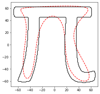
The DFT path certainly has the characteristics of the original image, but doesn't do a good job representing it. Lets increase the order to 100
order = 100
coef = coef_list(time, X, Y, order)
space = np.linspace(0,tau,300)
x_DFT = [DFT(t, coef, order)[0] for t in space]
y_DFT = [DFT(t, coef, order)[1] for t in space]
fig, ax = plt.subplots(figsize=(5, 5))
ax.plot(x_DFT, y_DFT, 'r--')
ax.plot(X, Y, 'k-')
ax.set_aspect('equal', 'datalim')
xmin, xmax = plt.xlim()
ymin, ymax = plt.ylim()
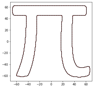
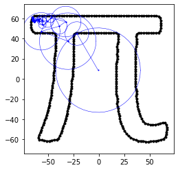
Almost indestinguishable from the original! What I love about this algorithm is it doesn't have any optimization algorithm to it or guessing methods, it is just a how well can I represent data given a base transformation. This is the power of Fourier transforms. And is highly related to how image compression works
The most beautiful and intuitive thing about the entire process is the visualization of the drawwing. All the math aside can't replace the imagery given by a series of circles stacked upon eachother to draw an image! Everytime it is brilliant!
anim = visualize(x_DFT, y_DFT, coef, order,space, [xmin, xmax, ymin, ymax])

#Change based on what writer you have
#HTML(anim.to_html5_video())
anim.save('pi.gif',writer='ffmpeg')
#anim.save('Pi.gif',writer='pillow')
Below are some other animations I've made with this same process:
Conclusion
So now we can take any image, do a fourier transform on it, and watch our little machine draw it in peace. I skipped over a lot of the math and wanted to just show the code, which you can download on my github. Maybe this is something that you would like to try yourself besides falling asleep at the math portion! If you want to learn more MyFourierEpicycles has a great description and further resources on how this works!
Cheers! -Q
Comments
comments powered by Disqus